

IRP Competitors: View Registered Teams.
Inventory Routing Problem (IRP) Statement
The Inventory Routing Problem (IRP) is one of the most challenging of the VRP variants, as it combines both inventory management and routing decisions into a single problem.
There are many different variants of the IRP, but this Challenge will consider a single variant that we believe to be both representative of the problem class and difficult because it includes both inventory and routing decisions and costs.
Input for IRP consists of locations for a depot and a set of n customers {1, …, n}, a time horizon consisting of T time periods {1, …, T}, and a fleet of M vehicles {1, …, M}. The depot is located at node 0. Each vehicle has capacity Q.
In each time period t, r0t units of a resource are made available at the depot, and rit units are consumed by customer i. Each node i in {0, …, n} begins with an initial inventory level of Ii0. Each customer i ∈ {1, …, n} must maintain an inventory level of at least Li and at most Ui and will incur a per-period cost of hi for each unit of inventory held. There is no maximum inventory level defined for the depot, but it cannot fall below 0, and there is per-period inventory holding cost of h0.
A matrix D specifies the distance (or some other cost) to travel between each pair of nodes.
The IRP is the problem of determining, for each time period t, the quantity to deliver to each customer i and the routes by which to serve those customers. An optimal solution is one that minimizes the total cost while assuring that constraints on vehicle capacity, vehicle routing, and node inventory levels are satisfied at all times. The total cost of a solution includes both the total of the inventory holding costs at all nodes (customers and depot) and the costs of the vehicle routes. A feasible solution must assure that:
- No customer stock-outs occur
- The depot has enough resource to meet deliveries in each period
- Each route begins and ends at the depot and honors the vehicle capacity constraint
- In each time period, a customer receives at most one delivery
This is the so-called Maximum Level (ML) replenishment policy, where any quantity can be delivered to the customers, provided that the maximum inventory level Ui is not exceeded and the minimum inventory level Li is satisfied.
Full Details for the IRP Challenge
The most complete and up-to-date information for the IRP competition is contained in the following document:
IRP Track Details & Rules [last updated: November 21, 2021]
Information is summarized on this webpage, but the IRP Track document is the definitive source for complete information.
IRP Algorithm Evaluation
Evaluation will take place in single evaluation round with all testing performed on the participant's own computer. Runs must be performed on a processor listed in PassMark.
Solvers must run on a single thread. If a solver solves linear relaxations or mixed integer linear programming problems, any commercial solver may be used as long as the commercial solver is run on a single thread.
A solver will be assessed based on the quality of the solutions obtained for each instance within a given amount of time. To mitigate the effect of processor speed, the time limit will be scaled for each individual processor. Solvers will be awarded points for their performance on each instance and ranked by the total number of points over all instances. The top three solvers, based on points, will be invited to present at the workshop, provided that the method is adequately described in an accompanying paper. Full details on scoring are contained in the IRP Rules document.
Additionally, the VRP Implementation Challenge committee will review all entries with respect to additional criteria such as novelty of the approach taken, simplicity, and versatility of a solver to work well on multiple different variants. We hope to recognize multiple entries for these attributes with invitations to present.
IRP Instances
IRP instances are provided in two zipped directories containing, respectively, small instances and large instances. [Download small IRP instances] [Download large IRP instances]
All instances are Euclidean.
In all instances, production at the depot and consumption at the customers is constant over all time periods. In this way, the test instances are less general than the problem statement given above and solvers may assume this fact.
Small instances have two possible values for the number of time periods, T, which will be either 3 or 6. T is 6 in all large instances.
Both the small and large instance sets are comprised of two subsets corresponding to instances with a low inventory cost and instances with a high inventory cost.
In all, there are 800 small instances and 240 large instances.
A description of the instances is provided in this PDF file. We note that two small instances do not have a feasible solution. They are Sabs5n5_5_L6 and Sabs5n5_5_H6.
Solution Cost:
The total cost of a solution is the sum of the total cost of travel and the total cost of inventory. The total travel cost is is based on Euclidean distance (see below). It is the total distance traveled by all vehicles over all time periods. The inventory cost is the sum of the cost of inventory at each customer node over all time periods plus the cost of inventory at the depot over all time periods. The inventory level is computed as described below.
Travel cost: All instances are Euclidean, so the node locations provided in the input file correspond to Euclidean coordinates for the nodes. To calculate the transportation cost, we will use a rounded Euclidean distance between consecutive customers i and j. That is calculated using the following formula to compute, dij,, the cost to travel from customer i to customer j.
dij = int((sqrt((xi - xj)2 + (yi - yj)2)+0.5)
where "sqrt" is the square root and "int" is a function truncating to the integer value.
Inventory cost: For each customer i, the inventory in period t is the inventory from time period t-1 plus the amount delivered in period t minus the amount consumed in period t. Letting qit be the quantity consumed by customer i in period t, the inventory level is:
Iit = Iit-1 + qit - rt
The figure below shows a simple flow of goods with associated inventories at a customer node over four periods.
For the depot, the inventory in period t is the inventory from period t-1 plus the amount produced in period t minus the total amount delivered to customers in period t.
Inventory costs are accounted for in all time periods {1, …, T}. Note that Inventory costs at time 0 are not considered.
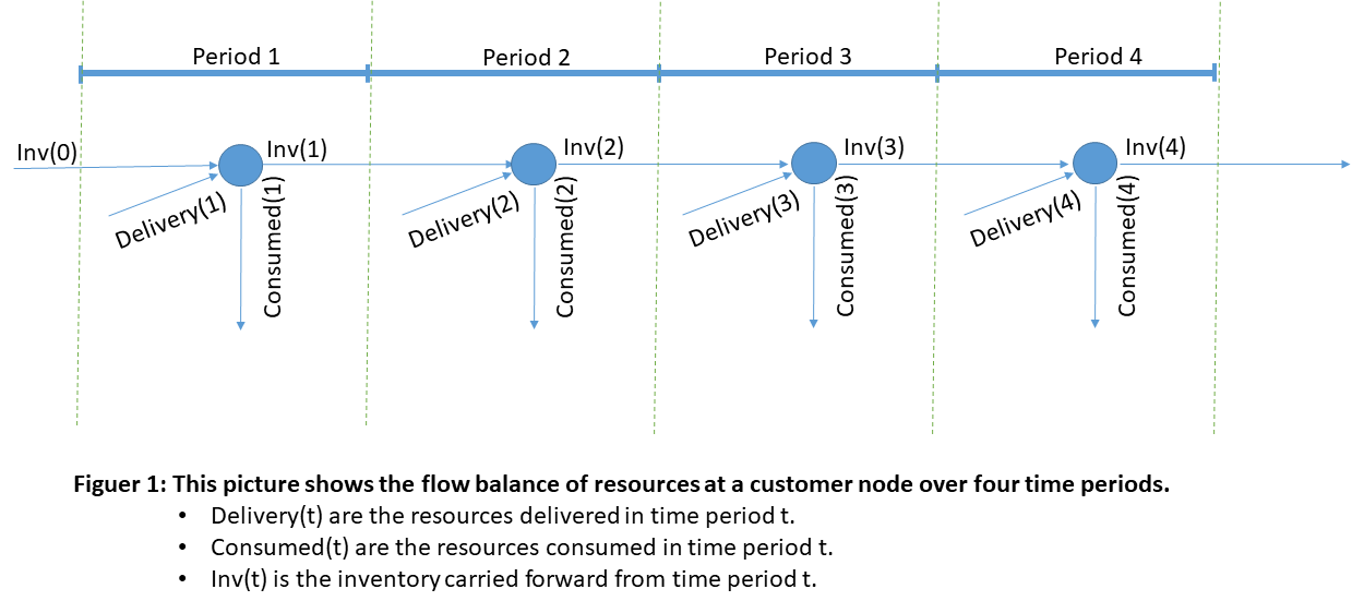
Inventory Bounds:
Although the picture above implies that consumption and delivery occur simultaneously in each time period, that would not be the case in practice. In the Challenge, we make the tacit assumption that delivery in period t occurs before consumption leading to the following constraints.
Lower Bounds: Iit ≥ Li
Upper Bounds: Iit-1 + qit ≤ Ui
Input File Format
Each IRP instance instance has the following format:
- The first line contains four parameters: the number of nodes including the depot (n+1), number of time periods T, vehicle capacity Q, and number of vehicles M.
- The second line describes the depot and provides: depot identifier (which is "0"), x coordinate, y coordinate, starting inventory level I00, daily production r0t, inventory cost h0.
- The n lines that follow each describes a customer and provides: customer identifier (i), x coordinate, y coordinate, starting inventory level Ii0, maximum inventory level Ui, minimum inventory level Li, daily consumption rit, inventory cost hi.
Output File Format
The name of the output file associated with an instance called "NAME" should be of the form out_NAME.txt.
The output file should be formatted such that the routes for each day are provided together, followed by the routes for the next day, and so on. For a given day, the route for each vehicle (1, … , M) is provided on a separate line. Routes for each time period should be numbered from 1 to M. Since each route begins and ends at the depot, each route provided in the output should begin and end at node 0. The customers on the route should appear in order, each followed by the amount of demand delivered to them on this route in parentheses. The last six rows of the file summarize the solution cost and time by providing:
- Total transportation cost
- Total inventory cost at customer locations
- Total inventory cost at the depot
- Total cost (sum of the three terms above)
- Processor (as listed in PassMark)
- Solution time (wall clock)
The format of the output is as follows:
Day 1
Route 1: 0 – customer ( quantity delivered ) – customer ( quantity delivered ) – … customer ( quantity delivered ) – 0
Route 2: 0 – customer ( quantity delivered ) – customer ( quantity delivered ) – … customer ( quantity delivered ) – 0
¦
Route M: 0 – customer ( quantity delivered ) – customer ( quantity delivered ) – … customer( quantity delivered ) – 0
Day 2
Route 1: 0 – customer ( quantity delivered ) – customer ( quantity delivered ) – … customer ( quantity delivered ) – 0
¦
Route M: 0 – customer ( quantity delivered ) – customer ( quantity delivered ) – … customer ( quantity delivered ) – 0
¦
Day T
Route 1: …
¦
Route M: …
Total transportation cost
Total inventory cost at customer locations
Total inventory cost at the depot
Total cost of the solution (which is the sum of the three terms above)
Processor
Solution time
A few points to clarify details about the format:
- Nodes in routes are separated by “blank_space – blank_space”
- The quantity delivered to each customer is reported after the customer node identifier this way: “customer_node blank_space parenthesis quantity blank_space parenthesis”.
The following is an example of example of a route that delivers 10 units to node 2 and 15 units to node 5:
0 – 2 ( 10 ) – 5 ( 15 ) – 0
It may be that not all vehicles make deliveries in every time period, but M routes must be output nonetheless. An empty route (not visiting any customers) is given this way:
0 - 0
Output files will be read and processed automatically. Therefore, files that do not comply with the format described above will be discarded.
Solution Checker
We are grateful to Stephan Beyer for making a feasibility checker available to participants. The code to verify IRP solutions is written in Python, and instructions for its use are provided in the associated README file.
Solution Values
A useful resource for checking the values of best known solutions (BKSs) is this spreadsheet that appears on the website of the OR Group at the University of Brescia.
We note that the spreadsheet includes information for all of the large instances but only 600 of the 800 small instances. It does not include the small instances having 6 time periods and more than 30 nodes.
You can map the Challenge instance name to the corresponding instance name in the spreadsheet by dropping the first character (either S or L) of the Challenge name, then dropping the final three characters (beginning with _), and then subtracting 1 from the final digit (corresponding to the number of vehicles).
As an example, the Challenge instance named Sabs1n5_2_L6 would map to the small instance abs1n5_1 that has a 6 time periods and large inventory costs in row 424 of the spreadsheet.
Finally, we note that the vehicle capacities in the Challenge instances differ slightly (in their rounding) from those of related instances in the literature (such as those of Coelho, L. C., Cordeau, J.-F., Laporte, G., Consistency in multi-vehicle inventory-routing, Transportation Research Part C 24(1) 270–287, 2012). As a result, solution values will differ.
Submission
When you are ready to submit either your solver output package (a zipped file) or your Challenge paper, you may do so from the Submissions page (which is part of the navigation menu on the right-hand side of this page).
No output is expected for the two infeasible instances Sabs5n5_5_L6 and Sabs5n5_5_H6.
Outputs are due January 30, 2022 and must be received by 23:59 Pacific Standard Time (UTC -8).
IRP Organizer(s)
Claudia Archetti (lead)
Questions
If you have questions, please email the organizers using this link.